BALD and BED: Connecting Bayesian active learning by disagreement and Bayesian experimental design
There is a deep connection between Bayesian experimental design and Bayesian active learning. A significant touchpoint is the use of the mutual information score as an acquisition function \(I(\xi) = \mathbb{E}_{p(\theta)p(y\mid \theta,\xi)}\left[H[p(\theta)] - H[p(\theta\mid y,\xi)]\right]\) which is also called the Expected Information Gain. In this equation, \(\theta\) are the Bayesian model parameters, \(y\) is the as yet unobserved outcome, and \(\xi\) is the design to be chosen. In the DBALD paper, Gal et al. introduced a means to estimate the mutual information acquisition function \(I(\xi)\) for active learning when using an MC Dropout-driven Bayesian neural network. In recent work on variational and stochastic gradient Bayesian experimental design, my collaborators and I studied estimators of the mutual information—including one in particular called Prior Constrative Estimation (PCE). Whilst the DBALD estimator and PCE look different on the surface, it turns out they have the same expectation and are almost identical: one is simply a Rao-Blackwellised version of the other. Which proves that the expectation of DBALD is always a lower bound on the true mutual information, which goes some way to explaining the stability of BALD as an acquisition function. Using this finding, we show that BALD actually has an upper bound “cousin” estimator.
Bayesian Active Learning by Disagreement
One of the computational challenges inherent in estimating mutual information directly is that it involves repeated estimation of posterior distributions \(p(\theta\mid y,\xi)\) for different simulated observations \(y\). To remove this particular bottleneck, Houlsby et al. used a rewriting of the mutual information score via Bayes rule
\[\begin{aligned} I(\xi) = H[p(y\mid \xi)] - \mathbb{E}_{p(\theta)}\left[ H[p(y\mid \theta,\xi)] \right]. \end{aligned}\]Whilst this is exactly equal to the original mutual information score, the new way of expressing \(I\) removes the requirement to estimate posterior distributions over \(\theta\). They termed this new rearrangement the Bayesian Active Learning by Disagreement (BALD) score.
Unfortunately, the story does not end with the BALD score because it still typically involves some intractable computations that must be estimated. For example, Houlsby et al. focused on approximations for Gaussian Process models.
The more recent work by Gal et al. estimated the BALD score in the context of Bayesian deep learning classifiers. In such a model, \(\theta\) represents the parameters of a classification model, and \(p(y\mid \theta,\xi)\) is a probability distribution over classes \(y\in\{c_1,\dots,c_k\}\). Computing \(p(y\mid \theta,\xi)\) involves a forward pass through the classifier with input \(\xi\) and parameters \(\theta\), the network generally ends in a softmax activation to produce a normalised distribution. To sample different values of \(\theta\), they employed Monte Carlo Dropout to approximate a BNN posterior. Given independent samples \(\theta_1,\dots,\theta_M\) from \(p(\theta)\), they proposed the following Deep BALD (DBALD) estimator of \(I(\xi)\)
\[\begin{aligned} I(\xi) \approx \hat{I}_\text{DBALD}(\xi) = H\left[ \frac{1}{M}\sum_{i=1}^M p(y\mid \theta_i,\xi) \right] - \frac{1}{M} \sum_{i=1}^M H[p(y\mid \theta_i,\xi)] \end{aligned}\]where \(H[P(y)] = -\sum_c P(y=c)\log P(y=c)\).
Notation: For comparison with the original paper, we used \(\theta\) in place of \(\bm{\omega}\), \(\xi\) in place of \(\mathbf{x}\), \(M\) in place of \(T\) and \(p(\theta)\) is used in place of \(q^*_\theta(\bm{\omega})\).
Prior Contrastive Estimation
In the context of stochastic gradient optimisation of Bayesian experimental designs, we also considered the mutual information score \(I(\xi)\) and the rearrangement used by BALD. We proved the following Prior Contrastive Estimation (PCE) lower bound on \(I(\xi)\)
\[\begin{aligned} I(\xi) \ge \mathbb{E}_{p(\theta_0)p(y\mid \theta_0,\xi)p(\theta_1)\dots p(\theta_L)}\left[ \log \frac{p(y\mid \theta_0,\xi)}{\frac{1}{L+1} \sum_{\ell=0}^L p(y\mid \theta_\ell,\xi)} \right] \end{aligned}\]and used this bound to optimise \(\xi\) by stochastic gradient when the design space is continuous. It works pretty well! One approach to estimate this bound using finite samples is the estimator
\[\begin{aligned} \hat{I}_\text{PCE-naive}(\xi) = \frac{1}{M} \sum_{m=1}^M \log \frac{p(y_m\mid \theta_{m0},\xi)}{\frac{1}{L+1}\sum_{\ell=0}^L p(y_m\mid \theta_{m\ell},\xi) }. \end{aligned}\]where \(y_m,\theta_{m0}\sim p(y,\theta\mid \xi)\) and \(\theta_{m\ell}\sim p(\theta)\) for \(\ell \ge 1\). However, we can also re-use samples more efficiently to give the estimator
\[\begin{aligned} \hat{I}_\text{PCE}(\xi) = \frac{1}{M} \sum_{m=1}^M \log \frac{p(y_m\mid \theta_{m},\xi)}{\frac{1}{M}\sum_{\ell=1}^M p(y_m\mid \theta_{\ell},\xi) }. \end{aligned}\]where \(y_m,\theta_m \sim p(y,\theta\mid \xi)\). (To check the expectation of this version matches the PCE bound with \(L=M-1\), we simply move the \(\mathbb{E}\) sign inside of the summation.) Finally, in our paper we discussed a speed-up that is possible when \(y\) is a discrete random variable taking values in \(\{ c_1,\dots,c_k \}\). In this case, we can integrate out \(y\) by summing over it, rather than by drawing random samples of \(y\). This method, called Rao-Blackwellisation, results in the estimator
\[\begin{aligned} \hat{I}_\text{PCE-RB}(\xi) = \frac{1}{M} \sum_{m=1}^M \sum_c p(y=c\mid \theta_m,\xi) \log \frac{p(y=c\mid \theta_{m},\xi)}{\frac{1}{M}\sum_{\ell=1}^M p(y=c\mid \theta_{\ell},\xi) }. \end{aligned}\]PCE and DBALD equivalence
We have looked at two parallel ways of approximating \(I(\xi)\). The interesting result is that the Rao-Blackwellised PCE estimator and the DBALD estimator are the same. We can see this by direct calculation
\[\begin{aligned} \hat{I}_\text{PCE-RB}(\xi) &= \frac{1}{M} \sum_{m=1}^M \sum_c p(y=c\mid \theta_m,\xi) \log \frac{p(y=c\mid \theta_{m},\xi)}{\frac{1}{M}\sum_{\ell=1}^M p(y=c\mid \theta_{\ell},\xi) } \\ &= \frac{1}{M} \sum_{m=1}^M \sum_c p(y=c\mid \theta_m,\xi) \log p(y=c\mid \theta_{m},\xi) - \frac{1}{M} \sum_{m=1}^M \sum_c p(y=c\mid \theta_m,\xi) \log\left(\frac{1}{M}\sum_{\ell=1}^M p(y=c\mid \theta_{\ell},\xi) \right) \\ &= -\frac{1}{M} \sum_{m=1}^M H[p(y\mid \theta_m,\xi)] - \frac{1}{M} \sum_{m=1}^M \sum_c p(y=c\mid \theta_m,\xi) \log\left(\frac{1}{M}\sum_{\ell=1}^M p(y=c\mid \theta_{\ell},\xi) \right)\\ &= -\frac{1}{M} \sum_{m=1}^M H[p(y\mid \theta_m,\xi)] - \sum_c \left(\frac{1}{M} \sum_{m=1}^M p(y=c\mid \theta_m,\xi) \right) \log\left(\frac{1}{M}\sum_{\ell=1}^M p(y=c\mid \theta_{\ell},\xi) \right)\\ &= -\frac{1}{M} \sum_{m=1}^M H[p(y\mid \theta_m,\xi)] + H\left[\frac{1}{M} \sum_{m=1}^M p(y\mid \theta_m,\xi) \right]\\ &= \hat{I}_\text{DBALD}(\xi). \end{aligned}\]A major consequence of this result is that, since we proved that the expectation of PCE is a lower bound on \(I(\xi)\), then the expectation of the DBALD score is a lower bound on the true mutual information score too. We also note that this estimator has been used by another paper in the context of Bayesian experimental design (there may be others out there too). I think we were the first to prove it is a stochastic lower bound.
New diagnostic for the DBALD score
Can these insights be used for anything? One advantage of making this connection is that we can bring certain diagnostics that were applied by in BED over to the active learning setting. In particular, in our paper we paired their PCE lower bound with a complementary upper bound on \(I(\xi)\) when doing evaluation. This provides a very useful diagnostic tool to tune the number of samples \(M\) used to compute the mutual information score. If the lower bound and upper bound are very close, we know that the difference between the DBALD score and the true mutual information must also be small. On the other hand, if the upper and lower bounds are far apart, then the DBALD score might not yet be close to the true mutual information.
The upper bound upper we used was the Nested Monte Carlo (NMC) estimator. For the discrete \(y\) case with Rao-Blackwellisation, the estimator is
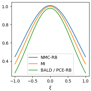
\[\begin{aligned} \hat{I}_\text{NMC-RB}(\xi) &= -\frac{1}{M} \sum_{m=1}^M \sum_c p(y=c\mid \theta_m,\xi) \log\left(\frac{1}{M-1} \sum_{\ell \ne m} p(y=c\mid \theta_\ell,\xi) \right) -\frac{1}{M} \sum_{m=1}^M H[p(y\mid \theta_m,\xi)]\\ &= \frac{1}{M} \sum_{m=1}^M H\left[p(y\mid \theta_m,\xi), \frac{1}{M-1} \sum_{\ell \ne m} p(y\mid \theta_\ell,\xi) \right] -\frac{1}{M} \sum_{m=1}^M H[p(y\mid \theta_m,\xi)] \\ &= \frac{1}{M} \sum_{m=1}^M \text{KL}\left[p(y\mid \theta_m,\xi) {\huge\|} \frac{1}{M-1} \sum_{\ell \ne m} p(y\mid \theta_\ell,\xi) \right] \end{aligned}\]where \(H[p,q]\) is the cross-entropy and \(\text{KL}[p\|q]\) is KL-divergence. The expectation of this mutual information estimator is always an upper bound on \(I(\xi)\), so NMC-RB is an upper bound “cousin” of DBALD. So both the DBALD score and the NMC-RB estimator converge to \(I(\xi)\) as \(M\to\infty\), but from opposite directions. We suggest NMC-RB as a diagnostic for the parameter \(M\).
BALD estimators for regression
The connection to PCE may also be helpful when considering regression models. The standard parametrisation of a Bayesian neural network for regression is for the output of the network with parameters \(\theta\) and input \(\xi\) to be the predictive mean \({\mu}\) and standard deviations \({\sigma}\) of a Gaussian \(y\mid \theta,\xi \sim N({\mu}(\theta,\xi), {\sigma}(\theta,\xi)^2)\). (It is normal for \(y\), \(\mu\) and \(\sigma\) to be vector-valued and for the Gaussian to have a diagonal covariance matrix.)
For the DBALD estimator for a regression model, the entropy of a Gaussian is known in closed form, so \(H[p(y\mid \theta_i,\xi)] = \tfrac{1}{2}\log\left(2\pi e \sigma(\theta_i,\xi)^2 \right)\). However, the entropy of a mixture of Gaussians \(H\left[ \frac{1}{M}\sum_{i=1}^M p(y\mid \theta_i,\xi) \right]\) cannot be computed analytically. Instead, we could estimate this mixture of Gaussians entropy using Monte Carlo by sampling \(i\in \{1,\dots,M\}\) uniformly, sampling \(y\) from \(p(y\mid \theta_i,\xi)\) and calculating the log-density at \(y\).
Despite the fact that we are using an analytic entropy for one term, and a Monte Carlo estimate for the other, it’s easy to see that this new estimator is a partially Rao-Blackwellised PCE estimator. (This can be proved starting from the definition of PCE.) That means all the existing facts, such as the estimator being a stochastic lower bound on \(I(\xi)\), carry over naturally to the regression case.
Conclusion
There are many overlaps between BED and BALD—in fact the DBALD score is equivalent to a Rao-Blackwellized PCE estimator. This proves that \(\mathbb{E}[I_{\text{DBALD}}(\xi)] \le I(\xi)\). It also reveals a “cousin” of the BALD score that is an upper bound on mutual information—it could be useful as a diagnostic.
Citation
This post is an edited version of Section 7.2 from my thesis. If you’d like to cite it, you can use
@phdthesis{foster2022thesis,
  Author = {Foster, Adam},
  Title = {Variational, Monte Carlo and Policy-Based Approaches to Bayesian Experimental Design},
  school = {University of Oxford},
  year={2022}
}
References
Adam Foster, Martin Jankowiak, Matthew O’Meara, Yee Whye Teh, and Tom Rainforth. A unified stochastic gradient approach to designing bayesian-optimal experiments. In International Conference on Artificial Intelligence and Statistics, pages 2959–2969. PMLR, 2020.
Yarin Gal and Zoubin Ghahramani. Dropout as a bayesian approximation: Representing model uncertainty in deep learning. In international conference on machine learning, pages 1050–1059. PMLR, 2016.
Yarin Gal, Riashat Islam, and Zoubin Ghahramani. Deep bayesian active learning with image data. In International Conference on Machine Learning, pages 1183–1192. PMLR, 2017.
Neil Houlsby, Ferenc Huszár, Zoubin Ghahramani, and Máté Lengyel. Bayesian active learning for classification and preference learning. arXiv preprint arXiv:1112.5745, 2011.
Benjamin T Vincent and Tom Rainforth. The DARC toolbox: automated, flexible, and efficient delayed and risky choice experiments using bayesian adaptive design. Retrieved from psyarxiv.com/yehjb, 2017.
Kenneth J Ryan. Estimating expected information gains for experimental designs with application to the random fatigue-limit model. Journal of Computational and Graphical Statistics, 12(3):585–603, 2003.