Optimising adaptive experimental designs with RL
This post follows up on a previous one which discussed the connection between Reinforcement Learning (RL) and Deep Adaptive Design (DAD). Here, I am taking a deeper dive into two 2022 papers that build off of DAD and use RL to train policies for adaptive experimental design: Blau et al. and Lim et al.. This is both a natural and interesting direction because training with RL removes some of the major limitations of DAD, such as struggling to handle non-differentiable models and discrete design spaces, and allows us to tap into advances in RL to optimise design policies.
Adaptive experimental design and DAD
Note: you can safely skip this section if you are already familiar with the DAD paper.
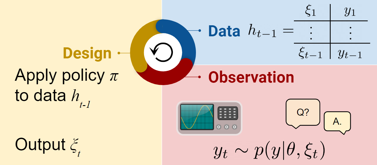
Adaptive design is an iterative procedure that consists of repeatedly
- designing experiments based on existing knowledge,
- running those experiments and obtaining experimental outcomes,
- updating knowledge based on data obtained so far.
In the Bayesian formulation, we have a model with prior \(p(\theta)\) and a likelihood \(p(y\mid\theta, \xi)\). The three steps of adaptive design are now
- selecting design \(\xi_t\) using past data \(h_{t-1} := (\xi_1,y_1),\dots,(\xi_{t-1},y_{t-1})\),
- obtaining outcome \(y_t\) by running an experiment with design \(\xi_t\),
- updating the posterior \(p(\theta\mid\xi_{1:t}, y_{i:t})\).
In DAD, the choice of \(\xi_t\) is made by a neural network design policy \(\pi\).
This DAD policy is trained by gradient descent to maximize a lower bound on the total expected information gain from the sequence of experiments \(h_T = (\xi_1,y_1),\dots,(\xi_T,y_T)\). This lower bound is called sequential prior contrastive estimation (sPCE)
\[\mathcal{I}_T(\pi) = \mathbb{E}_{p(\theta)p(h_T\mid\theta,\pi)} \left[ \log \frac{p(h_T\mid\theta,\pi)}{p(h_T\mid \pi) } \right] \ge \text{sPCE}_{T,L}(\pi) = \mathbb{E}_{p(\theta_{0:L})p(h_T\mid\theta_0,\pi)} \left[ \log \frac{p(h_T\mid\theta_0,\pi)}{\frac{1}{L+1} \sum_{\ell=0}^L p(h_T\mid\theta_\ell,\pi) } \right].\]The policy network is designed to account for the permutation invariance of experimental histories: these are represented using a permutation invariant neural representation. This was an innovation compared to earlier work, which explicitly computed the posterior \(p(\theta\mid\xi_{1:t},y_{1:t})\) at each step. The policy is updated by gradient descent on the policy parameters. Typically, this is by end-to-end backprop, which is valid for reparametrisable likelihoods. The alternative is to use a score function gradient estimator; this is necessary, for example, when \(y\) is discrete.
New direction: using RL to train the design policy
In my previous post, I discussed how the sequential experimental design problem can naturally be cast as Bayes Adaptive Markov Decision Process. In February-March 2022, new papers hit arXiv using RL to train design policies. In this post I will talk about the details of those papers, specifically Blau et al. (2022) and Lim et al. (2022), because these are the papers that most directly use ideas from DAD, and hence are closest to my own expertise. I have therefore set aside important papers such as Huan & Marzouk (2016), Shen & Huan (2021) and Asano (2022). For the papers I will tackle in this post, I want to pre-emptively apologise for any errors of understanding that I may make.
‘Optimizing Sequential Experimental Design with Deep Reinforcement Learning’ by Blau et al.
This paper kicks off by formulating the adaptive experimental design problem in the language of RL. Blau et al. formulate the problem as a Hidden Parameter MDP (HiP-MDP). The HiP-MDP is an extension of the MDP in which different RL tasks are encoded by different values of a latent variable \(\theta\). The transition function and reward function can then depend on \(\theta\). A HiP-MDP is therefore an MDP once we condition upon the value of \(\theta\). The HiP-MDP is a nice formulation I hadn’t seen before that seems almost custom-made for the sequential experimental design problem. In this set-up, the states are histories \(h_t\), the actions are designs \(\xi_t\), the hidden parameters are \(\theta_{0:L}\) and the transition function is the likelihood \(p(y\mid \theta_0,\xi)\). The policy \(\pi\) operates on the history states \(\xi_{t+1} = \pi(h_t)\), and by including \(\theta_{0:L}\) in the hidden parameters, the sPCE objective can be computed as the reward.
Exactly formulating the problem in the language of RL is a slightly finicky exercise! For instance, the sequence \((\xi_1,y_1),(\xi_2,y_2),\dots\) is not Markovian; the sequence \(h_1,h_2,\dots\) is Markovian, but to evaluate the sPCE objective you also need access to \(\theta_{0:L}\), so should these form part of the state or part of a stochastic reward? I previously described the adaptive experimental design problem as a BAMDP; it’s also possible to describe it as a pure MDP with an extended state space. I like the HiP-MDP as it seems to most naturally match the experimental design set-up.
State representation and reward
As in DAD, Blau et al. use permutation invariant state representations of the form
\[B_t = \sum_{\tau=1}^t ENC_\psi(\xi_\tau,y_\tau)\]where \(ENC_\psi\) is a neural net encoder. The policy has access to the state only via this neural state representation. This permutation-invariant state representation is quite useful because it side-steps challenges with the other two natural possibilities: computing the belief states \(p(\theta \mid h_t)\) explicitly is valid but computationally burdensome, using the histories \(h_t\) directly as states is awkward because the dimension of the state changes at each time step and the permutation invariance has to be explicitly learned.
Blau et al. base their reward on the sPCE objective from DAD. Again, this side-steps the simpler but less scalable alternative used, e.g. in Huan & Marzouk (2016), which is to estimate the posterior \(p(\theta \mid h_T)\) and then take the information gain \(H[p(\theta)] - H[p(\theta \mid h_T)]\) as the reward. This choice, combined with the neural state representation, has the distinct advantage of avoiding any explicit computation of posteriors during training and deployment.
Blau et al. point out that there are several RL reward structures that can be devised based on sPCE. The simplest terminal-only form of the reward is to have \(0\) reward up to time \(T-1\), and then a reward of
\[g(\theta_{0:L},h_T) = \log \frac{p(h_T\mid\theta_0,\pi)}{\frac{1}{L+1}p(h_T\mid\theta_\ell,\pi)}\]at time \(T\). This sparse reward can present problems for RL algorithms. An equivalent form is to use the step-by-step rewards \(r_t = g(\theta_{0:L},h_t) - g(\theta_{0:L},h_{t-1})\). This telescopes nicely to assign the correct reward to the sequence of designs and observations, whilst providing a reward signal at every step. Blau et al. adopt the step-by-step reward, and give an efficient way to compute it. They compare experimentally to the terminal-only reward, and show that step-by-step rewards are better across the board.
Of course, it is necessary to prove that using these rewards does lead to the correct expected return. This is taken care of in Theorems 1 and 2.
RL stuff
Explore-exploit
In Blau et al., the design policy is stochastic, meaning that the design \(\xi_t\) is sampled from a distribution \(p(\xi_t \mid \pi(h_{t-1}))\). In Blau et al., the distribution is Gaussian when designs are continuous. As the authors say, exploration is important for RL and modern RL algorithms incorporate many tricks to enable good exploration. Incorporating exploration can avoid the policy becoming trapped in local optima.
It remains an open question (at least for me) whether a stochastic policy would also be beneficial for the original DAD formulation using stochastic gradient optimisation. Whilst adding explicit exploration is the norm in RL, it certainly is not the norm when optimising with stochastic gradient descent, even when we know the objective is not convex. One reason for this is that, by using gradient methods, we can “see” policies in an infinitesimal neighbourhood of the current policy. We also know that the optimal policy is not stochastic (from Lindley, 1956), so this would only ever be a method for training a policy that is deterministic at the end.
Choice of RL algorithm
The authors went with Randomized Ensembled Double Q-learning (REDQ) as their RL algorithm of choice, but didn’t dig much into the choice. I’m still a bit in the dark about whether this is a particularly good algorithm to have chosen.
Putting everything together
In total then, Blau et al. solve an RL problem using REDQ with
- history states \(h_t\) with fixed-dimensional permutation-invariant neural representation \(B_t\) which are exposed to the policy,
- actions are experimental designs \(\xi_t\),
- the policy samples \(\xi_t \sim p(\xi_t \mid \pi(B_{t-1}))\),
- the transition dynamics are given by \(y_t \sim p(y \mid \theta_0,\xi_t)\) and \(h_t = h_{t-1} \cup (\xi_t,y_t)\),
- the discount factor is \(\gamma=1\),
- the reward for moving from \(h_{t-1}\) to \(h_t\) is \(r_t = g(\theta_{0:L},h_t) - g(\theta_{0:L},h_{t-1})\), which depends on all the \(\theta_{0:L}\).
Experiments
One thing that the experiments demonstrated very nicely is that the RL version of DAD is widely applicable: it works for discrete design spaces and non-differentiable models with no extra effort!
Source location
This model was originally used in the DAD paper. It represents an experimenter trying to locate two hidden sources that are emitting a signal that decays with an inverse square law. Specifically, we have two source locations \(\theta^{(1)},\theta^{(2)} \sim N(0,I_d)\) and a design \(\xi \in \mathbb{R}^d\). The likelihood is given by \(\log y \sim N(\log \mu(\theta,\xi), \sigma^2)\) where
\[\mu(\theta,\xi) = b + \frac{1}{m + \|\theta^{(1)} - \xi \|^2}+ \frac{1}{m + \|\theta^{(2)} - \xi \|^2}.\]Here is a visualisation of DAD applied to this problem
In Blau et al., they compare the new RL approach against DAD, showing that RL has a decent edge for this problem with a time horizon \(T=30\). (It would be great to see a comparable animation for the RL policy to see whether it has an qualititative differences.)
Constant elasticity of substitution
Constant elasticity of substitution was studied in SG-BOED. This model comes from behavioural economics, and the experiment modelled is one in which a human participant has to examine two offered baskets of goods, e.g. two apples and one banana versus two bananas, and then respond on a sliding 0-1 scale indicating which they prefer. The aim of the experiment is to learn the participant’s preferences for the different items, as well as a parameter \(\rho\) which (roughly speaking) indicates how much the participant prefers a “balanced” basket of items.
In this model, \(y\) is only differentiable over part of its range due to clipping, requiring specialist treatment for DAD, but presenting no issues for RL. Here, there are substantial qualitative differences between DAD designs and RL designs- it appears RL explores the design space much more than DAD. For example, Figure 3 shows that DAD designs often cluster around a single value across different experiments, whilst the RL designs take a much wider range of values. The RL algorithm also performs best in terms of total EIG.
Predator-prey
This model was previously tackled with an SMC approach. Here, we have a discrete design space so cannot directly be solved with DAD. In this model, predators eat prey, meaning that prey population numbers change according to a differential equation
\[\frac{dN}{dt} = -\frac{aN^2}{1 + aT_h N^2}\]where \(\theta = (a, T_h)\) are the model parameters that have to be learned. The design \(\xi\) is the initial prey population, and the observation \(y\) is the number of prey remaining at some time \(\mathcal{T}\). This is sampled from a binomial distribution with probability \(N_\mathcal{T} / \xi\).
Interestingly, adaptive RL-based optimisation doesn’t do any better here than myopic design using SMC. For adaptive experiments, the success of the greedy strategy can depend on the ability to compute intermediate posterior distributions accurately. My hunch is that SMC is a good practical choice here because the posteriors on 2-dimensional \(\theta\) are quite easy to approximate. The authors also suggest that the state representations could be to blame. This could be tested empirically by increasing the representation dimension, increasing the encoder network size or using extra tricks like self-attention.
Summing up
The results are very promising. I was curious how difficult training was, as folklore tells us that deep RL is ‘very hard to train’. I was glad to see this work published at ICML 2022!
‘Policy-Based Bayesian Experimental Design for Non-Differentiable Implicit Models’ by Lim et al.
This paper tackles a more challenging problem setting by incorporating some of the generalisations that we examined in the iDAD paper, namely
- experiments are not assumed to be permutation invariant, as we replace the likelihood \(p(y\mid \theta,\xi)\) with a history-dependent likelihood \(p(y\mid \theta,\xi_t,h_{t-1})\),
- the likelihood is not assumed to be tractable, making this an implicit likelihood scenario.
However, unlike iDAD, Lim et al. also assume that the simulator that creates samples from \(p(y\mid \theta,\xi_t,h_{t-1})\) is not differentiable. This differentiability was a key assumption in iDAD that enabled gradient-based optimisation of the design policy.
Initially, the authors set up the problem in the language of RL, choosing this time to formulate the problem as a Partially Observed MDP (POMDP). The set-up is similar to what we have seen already with Blau et al., except that \(\theta_{0:L}\) now forms part of the partially observed state. There is an important point here that breaking the permutation invariance of experiments does not fundamentally alter the Markovian structure provided the additional dependence of \(p(y\mid \theta,\xi_t,h_{t-1})\) is only on the observed history \(h_{t-1}\). (We have now seen the sequential experimental design problem formulated as a BAMDP, HiP-MDP and a POMDP. I don’t think the distinction between these is important: the proofs are all roughly the same.)
Rewards with implicit likelihood
Lim et al. take their cue from iDAD and base a reward function on the InfoNCE lower bound
\[\mathcal{I}_T(\pi) = \mathbb{E}_{p(\theta)p(h_T\mid\theta,\pi)} \left[ \log \frac{p(h_T\mid\theta,\pi)}{p(h_T\mid \pi) } \right] \ge \text{InfoNCE}_{T,L,\psi}(\pi) = \mathbb{E}_{p(\theta_{0:L})p(h_T\mid\theta_0,\pi)} \left[ \log \frac{\exp(U_\psi(h_T,\theta_0))}{\frac{1}{L+1} \sum_{\ell=0}^L \exp(U_\psi(h_T,\theta_\ell)) } \right].\]This is actually quite a significant change from previous approach using sPCE. In Blau et al., the rewards based directly on sPCE do not have their own parameters: they are simple functions of \(\theta_{0:L}\) and \(h_T\). In contrast, the InfoNCE objective is a variational objective: it contains the learned parameter \(\psi\) for the critic \(U_\psi\). The reward only comes close to the true EIG when \(\psi\) is optimised. The critic can also be used to estimate the posterior on \(\theta\) at the end of the experiment.
Note: The critic \(U_\psi\) that estimates an unnormalised joint density is quite distinct from any critic that might be involved in the RL algorithm (which could be confusing when using actor-critic algorithms).
Similarly to Blau et al., Lim et al. point out that the most obvious way to apply the InfoNCE objective within RL would be to use terminal-only (i.e. sparse) rewards. Looking ahead to the experiments for a second, this sparse reward formulation appears to fail catastrophically when combined with InfoNCE (Figure 1 in the paper). Instead, a step-by-step reward is more effective. The step-by-step (i.e. dense) rewards are defined similarly to Blau et al., but using InfoNCE instead of sPCE:
\[r_t = g_{L,\psi}(h_t, \theta_{0:L}) - g_{L,\psi}(h_{t-1}, \theta_{0:L})\]where
\[g_{L,\psi}(h_t,\theta_{0:L}) = \log \left[ \frac{\exp(U_\psi(h_t,\theta_0))}{\frac{1}{L+1} \sum_{\ell=0}^L \exp(U_\psi(h_t,\theta_\ell)) } \right] .\]Training the policy and the critic
Unlike in Blau et al., the implicit likelihood settings has this problem of having to learn the policy and the critic \(U_\psi\) at the same time. When optimising everything end-to-end with gradient descent in iDAD, we interpreted this simply as gradient descent on an enlarged set of parameters. When updating policy and critic with different algorithms (RL, gradient descent), I was concerned that something might go wrong. Algorithm 1 from Lim et al. suggests everything is fine: the policy is updated using TD3 and critic is updated with some gradient steps, and we simply alternate.
There is a subtlety tucked away in the appendix: the critic, \(U_\psi\), is dealt with using a ‘target network’. This is quite a standard idea in RL. The target network is essentially a lagged version of \(\psi\) and this is used to give rewards to train the policy. This is expected to give better stability to the RL training. Overall, I felt that this paper has only begun to stratch the surface of an interesting question that is clearly relevant to experimental design: how do we learn the reward at the same time as the policy?
In Lim et al., the choice of RL algorithm was TD3. This algorithm requires the training of the policy \(\pi\) and a Q-network \(Q_\omega\). As with the other paper, I was left a little mystified about why exactly this algorithm was chosen. Also like Blau et al., the policy is stochastic through the addition of some Gaussian noise to encourage exploration.
Finally, the authors mentioned that using an encoding of the history as an input to the policy (either a permutation-invariant attention-based encoding, or a LSTM encoding) is not as effective as simply concatenating the whole history and padding unseen experiments with zeros. This means that the state representation is of fixed dimension \(T(\text{dim}(y) + \text{dim}(\xi))\), and the representation of \(h_t\) with \(t<T\) simply has zeros in the last \((T-t)(\text{dim}(y) + \text{dim}(\xi))\) positions. This is something we actually tried out during the iDAD project, but didn’t find it to be particularly effective. Perhaps the encoder networks here were too weak and acted as a bottleneck. Using the concatenation approach cuts out a piece of complexity and lets the policy and Q-network do the work themselves. It’s also possible that, once the permutation invariance is broken, the main gains from using a neural representation of the history are negated.
Experiments
First, the authors looked at the Location Finding model, but unlike Blau et al., they treated this as an implicit likelihood model by denying themselves access to the likelihood when training. As expected, this is a more difficult problem. In particular, whilst Blau et al. reported that they could outperform DAD using RL, Lim et al. are not able to get past DAD. It seemed like RL-DAD could be doing better than iDAD. (It was not typical to see only the sNMC upper bounds in Table 1, usually we present both upper and lower bounds on total EIG which can give more definite conclusions.) Figure 1 drives home the point that sparse rewards really do not work for RL when we are also learning \(U_\psi\). For the Susceptible-Infected-Recovered (SIR) model that was studied in iDAD, the RL-DAD approach appears to have comparable but no better performance than iDAD.
I was most interested by the Cartpole experiment. Cartpole is an environment that is more often seen in RL papers. It is a simulator of a physical system in which a pole is attached at one end to a freely sliding cart. Typically, the RL agent has to learn how to keep the pole balanced above the cart. But it can also be interpreted as an experimental design problem in which the cart is manipulated to uncover the unknown physical parameters of the system: the mass \(m\) of the cart and the coefficient of friction \(\mu\) between the cart and the pole. By using a non-differentiable RL Gym implementation of this environment, we have a genuine non-differentiable simulator without a known likelihood. Here, RL-DAD does well and does substantially better than the most realistic alternative algorithm, which is MINEBED-BO.
Conclusions
These two papers demonstrate that using RL algorithms in the DAD/iDAD framework is effective for training experimental design policies in both explicit and implicit likelihood settings.
Where might using RL be most useful? My hunch is that we can see these approaches being most useful for:
- Discrete design and mixed discrete-continuous design problems. RL is well-optimised for environments where there are a small number of discrete actions available at each step. Many experimental design problems naturally incorporate discrete decisions, e.g. in experimental design for causal discovery. Another very natural area to consider is pool-based active learning. This is a well-studied experimental design problem with discrete actions; the issue here is that the design space is very large (perhaps tens of thousands of unlabeled examples in the pool), so it isn’t clear if RL would be a sensible choice here, or indeed if non-greedy experimental design can be expected to have an edge over the usual greedy strategy.
- Long experiments. We haven’t yet properly explored adaptive experiments with hundreds of adaptive steps. It is likely that the standard gradient-based training will degrade for very long experiments. Unfortunately, both the sPCE and InfoNCE objectives will also degrade here, so RL is only one piece of a possible solution. One idea is to draw contrastive samples, not from the prior, but from a learned proposal distribution- this gives rise to the sACE and sLACE bounds (see DAD: Appendix B, iDAD: Appendix B). When using these bounds, there is yet another component - the proposal - that must be jointly trained along with everything else. Digging deeper into the problem of interleaving RL updates with other updates to learn the proposal seems relevant in this case.
Finally, there is the question of where policy-based experimental design algorithms are most important in general. This is one reason I found the cartpole environment interesting: it represents a dynamically evolving environment that cannot be “paused” once experimentation begins and therefore requires very rapid design decisions.
References
Blau, T., Bonilla, E. V., Chades, I., & Dezfouli, A. (2022). Optimizing Sequential Experimental Design with Deep Reinforcement Learning. In International Conference on Machine Learning (pp. 2107-2128). PMLR.
Lim, V., Novoseller, E., Ichnowski, J., Huang, H., & Goldberg, K. (2022). Policy-Based Bayesian Experimental Design for Non-Differentiable Implicit Models. arXiv preprint arXiv:2203.04272.
Adam Foster, Desi R Ivanova, Ilyas Malik and Tom Rainforth (2021). Deep Adaptive Design: Amortizing Sequential Bayesian Experimental Design. In Proceedings of the 38th International Conference on Machine Learning, pages 3384-3395. PMLR.
Ivanova, D. R., Foster, A., Kleinegesse, S., Gutmann, M. U., & Rainforth, T. (2021). Implicit deep adaptive design: policy-based experimental design without likelihoods. Advances in Neural Information Processing Systems, 34, 25785-25798.
Asano, H. (2022). Sequential Bayesian experimental designs via reinforcement learning. arXiv preprint arXiv:2202.07472.
Xun Huan and Youssef M Marzouk (2016). Sequential bayesian optimal experimental design via approximate dynamic programming. arXiv preprint arXiv:1604.08320.
Shen, W., & Huan, X. (2021). Bayesian sequential optimal experimental design for nonlinear models using policy gradient reinforcement learning. arXiv preprint arXiv:2110.15335.
Lindley, D. V. (1956). On a measure of the information provided by an experiment. The Annals of Mathematical Statistics, 27(4), 986-1005.
Doshi-Velez, F., & Konidaris, G. (2016). Hidden parameter markov decision processes: A semiparametric regression approach for discovering latent task parametrizations. In IJCAI: proceedings of the conference (Vol. 2016, p. 1432). NIH Public Access.
Moffat, H., Hainy, M., Papanikolaou, N. E., & Drovandi, C. (2020). Sequential experimental design for predator–prey functional response experiments. Journal of the Royal Society Interface, 17(166), 20200156.