Stochastic-gradient Bayesian Optimal Experimental Design with Gaussian Processes
A couple of people have asked me how Gaussian Process (GP) models can be incorporated into the framework of Stochastic Gradient Bayesian Optimal Experimental Design (SGBOED) and Deep Adaptive Design (DAD). Where a lot of older work on experimental design and particularly Bayesian optimisation only works for GP models, it seems prima facie that SGBOED does not work for GPs or any nonparametric Bayesian models. In this post, I’ll show conceptually that SGBOED works with GPs. There is also a Pyro code example. In a subsequent post I will look into more exotic models that incorporate GPs, as well as adaptivity and other objective functions for learning designs.
A quick recap on SGBOED
The SGBOED algorithm is a gradient-based approach to finding experimental designs that maximise the expected information gain (EIG) between the experimental data and the model’s parameters. Denote the model parameters \(\theta\), the prior \(p(\theta)\), design \(\xi\), the experimental outcome \(y\) with likelihood model \(p(y\mid\theta,\xi)\). The simplest objective function we proposed, that should be maximised with respect to \(\xi\), was the prior contrastive estimation (PCE) objective
\[I_\textrm{PCE}(\xi) = \log \frac{p(y\mid\xi, \theta_0)}{\frac{1}{L+1} \sum_{\ell=0}^L p(y\mid\xi, \theta_\ell)}\]where \(\theta_{0:L} \sim p(\theta)\) and \(y \sim p(y\mid\theta_0,\xi)\).
In the SGBOED paper, we showed that the expectation of this quantity is a lower bound on the true EIG.
The problem with GP models
In the parametric Bayesian model that we considered in the SGBOED paper, the target of inference is the set of all model parameters \(\theta\). This is a finite dimensional vector with a prior that we can sample quite easily and explicitly. Once we introduce GPs into the mix, the target of inference needs to be more carefully handled.
To be concrete, let us begin with the simple regression model
\[\begin{aligned} f &\sim \mathcal{GP}(0, k(\cdot, \cdot)) \\ y | f,\xi &\sim N(f(\xi), \sigma^2). \end{aligned}\]Now we have introduced the random function \(f\), the GP kernel \(k\) and a fixed and known observation variance \(\sigma^2\). In this post, let us also assume that the kernel function is fixed and known. In this case, the random function \(f\) now plays the role of the \(\theta\) in the earlier model. In particular, the target of inference is the unknown function \(f\), which is infinite dimensional. Unlike in the parametric case, we cannot represent \(\theta\) explicitly, so where we have \(\theta_{0:L} \sim p(\theta)\) in the SGBOED algorithm, what should be done in the GP case?
Fortunately, the PCE objective only involves terms of the form \(p(y|\xi, \theta)\) and \(y\) only depends on \(f\) through the finite-dimensional \(f(\xi)\). Thus, we can sample only \(f_0(\xi), f_1(\xi), \dots, f_L(\xi)\) from the prior (these end up being independent Gaussians) and then evaluate the PCE objective as normal
\[I_\textrm{PCE}(\xi) = \log \frac{p(y|f_0(\xi))}{\frac{1}{L+1} \sum_{\ell=0}^L p(y|f_\ell(\xi))}.\]Similarly, and more interestingly, if we allow \(\xi\) to have a batch dimension, say \(\xi^{(b)}\) are different components of a batch design for \(b=1,\dots,B\), and we use the model
\[\begin{aligned} f &\sim \mathcal{GP}(0, k(\cdot, \cdot)) \\ y^{(b)} | f,\xi &\sim N(f(\xi^{(b)}), \sigma^2) \text{ independently over } b, \end{aligned}\]then we should now jointly sample \(f_i(\xi^{(1)}), \dots, f_i(\xi^{(B)})\) in place of sampling \(\theta_i\) in the original PCE algorithm. This is because \(y\) (which is now a \(B\)-dimensional vector) only depends on \(f\) through \(f(\xi^{(1)}), \dots, f(\xi^{(B)})\).
Comments
Never do this in practice
The purpose of this example is to plug a conceptual hole in the SGBOED theory. It has to come with a very hefty caveat: you should never use SGBOED with a basic GP regression model in practice. This is because the EIG, of which PCE is a sample-based lower bound, can simply be computed in closed form for this model. If you’re unfamiliar with how to derive this closed form, the idea (for the batch design case) is to use \(\text{EIG} = H[p(y)] - \mathbb{E}[H[p(y\mid f)]]\). Then we use the two following observations
- \(H[p(y\mid f)]\) is a constant that we can ignore. If you want to evalute the exact MI, you can compute it using the fact \(y\mid f\) are independent Gaussians of variance \(\sigma^2\),
- \(H[p(y)]\) is the entropy of a Multivariate Gaussian. The covariance matrix can be computed using \(\xi\) and the kernel \(k\) and the entropy can be evaluated using the formula.
These formulas only hold for the basic model though; in a later post we will see more complex models where some kind of EIG estimation is necessary.
Bayesian Active Learning by Disagreement
The observation that you can get at the EIG involving an infinite dimensional quantity, like a GP, by considering likelihoods of the form \(p(y\mid f(\xi))\) is one of the main ideas of the original Bayesian Active Learning by Disagreement (BALD) paper. Indeed, the formula \(\text{EIG} = H[p(y)] - \mathbb{E}[H[p(y\mid f)]]\) is often referred to as BALD. The BALD paper also has some neat stuff on EIGs for classification (which are not covered by an explicit formula like the regression case).
Code
A runnable version of the code, plus installation instructions, is available in a standalone repo.
The code is based on the existing DAD repo and is written using the Pyro probabilistic programming language. This repo already implements the PCE objective and the wrappers needed to get Pyro models working well with BOED. We can import these
from oed.primitives import observation_sample, compute_design, latent_sample
from oed.design import OED
from contrastive.mi import PriorContrastiveEstimation
Now let’s start writing a model. Our GP will be defined on the space \((-1, 1)^2\) and we will use a batch design, so \(\xi \in (-1, 1)^{2 \times B}\) and \(y \in \mathbb{R}^B\). We will use the RBF kernel \(k(\xi^{(b)}, \xi^{(b')}) = \exp\left(-\frac{1}{2 \ell ^ 2}\|\xi^{(b)} - \xi^{(b')}\|^2\right)\) where \(\ell\) is the lengthscale.
import torch
import pyro
import pyro.distributions as dist


class RBFGaussianProcessModel:
    """Implements a Pyro GP model suitable for SGBOED."""

    def __init__(self, batch_size=6, dim=2, lengthscale=1.0, device="cuda:0"):
        self.batch_size = batch_size
        self.dim = dim
        self.lengthscale = lengthscale
        self.device = device

    def model(self):

        # The design is a pyro.param that is transformed to [-1, 1]^{dim}
        design = pyro.param("design", torch.empty([self.batch_size, self.dim], device=self.device).normal_())
        design = torch.tanh(design)

        # Evaluate the RBF kernel between each design point in the batch design
        cov = torch.exp(-(design.unsqueeze(-3) - design.unsqueeze(-2)).pow(2).sum(-1) / (2 * self.lengthscale ** 2))
        # Add tiny diagonal variance for stability. This is *not* observation noise
        cov = cov + 1e-7 * torch.eye(cov.shape[-1])

        # The `latent_sample` instruction overrides pyro.sample and tags the sample as a model latent
        means = latent_sample("means", dist.MultivariateNormal(torch.zeros(self.batch_size, device=self.device), cov))
        # The `observation_sample` instruction similarly adds a tag to this sample site for an experimental outcome
        # The observation variance is set to 1.0

        # The `.to_event(1)` tells Pyro that y is vector of dimension `self.batch_size`
        # By adding `.to_event(1)`, when Pyro computes the conditional log-likelihood of y, it sums over the individual
        #  batch components of `y`, which is correct, rather than returning a separate log-likelihood for each
        #  component of `y`, which would give an incorrectly shaped likelihood tensor
        y = observation_sample("y", dist.Normal(means, 1.0).to_event(1))
        return y
The trick here is to treat means, which is exactly \(f_i(\xi^{(1)}), \dots, f_i(\xi^{(B)})\), as the latent variable of the model.
Finally, we can add some standard code to run the stochastic gradient algorithm. (This is a simplified version of code that you can find on the DAD repo).
from tqdm import trange
import numpy as np

from pyro.infer.util import torch_item

def single_run(seed, num_steps=20000):

    pyro.clear_param_store()
    pyro.set_rng_seed(seed)

    pce_loss = PriorContrastiveEstimation(10, 100)
    gp_model = RBFGaussianProcessModel(batch_size=9, device="cpu")  # small tensors may be faster on CPU

    optimizer = pyro.optim.Adam(optim_args={"lr": 0.003, "weight_decay": 0, "betas": (0.5, 0.9)})
    oed = OED(gp_model.model, optimizer, pce_loss)

    loss_history = []
    t = trange(1, num_steps + 1, desc="Loss: 0.000 ")
    for i in t:
        loss = oed.step()
        loss = torch_item(loss)
        # The loss here is not quite PCE, it is log(L+1) - PCE
        # Thus, lower loss => higher PCE, loss = 0 implies PCE is maximised at log(L+1)
        t.set_description("Loss: {:.3f} ".format(loss))
        loss_history.append(loss)

    final_design = np.tanh(pyro.param("design").cpu().detach().numpy())


if __name__ == "__main__":
    seed = np.random.randint(100000)
    single_run(seed)
If you run the full script it creates a number of plots. One is a loss curve like the following.
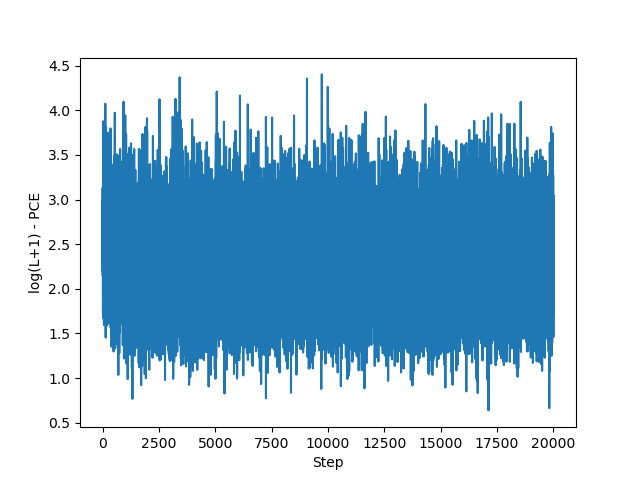
You can see that the loss is quite noisy and doesn’t seem to make much progress. But don’t let that fool you: the gradients can still provide good signal as evidenced by the movement of the design points.
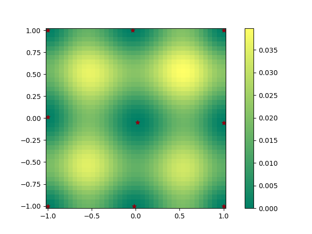
After 20k steps, the design should settle into a rather regular pattern that “spaces out” points. There are local optima in this problem and you will likely get a few different solutions with different random seeds.
This plot shows the final design I got (dark stars). I also plotted the predictive variance in \(f(\xi)\) at different points on the domain after conditioning the GP on data using design \(\xi\). The predictive variance in the vanilla GP does not depend on the values of \(y\) (do not expect this to hold for more exotic models). For comparison, the predictive variance in the prior is 1.
Costs and benefits of Pyro
Pyro is a tricky language to get the hang of, partly because of the strict rules it imposes on tensor shapes (among other things). However, Pyro does provide some neat advantages. Firstly, you do not have to write a new implementation of the PCE objective for every new model. Secondly, the simulator and the likelihood model must be consistent by design. This is something that could easily go wrong if you wrote your own implementation. Of course, it would be possible to redo this exercise in pure PyTorch.
References
Adam Foster, Martin Jankowiak, Matthew O’Meara, Yee Whye Teh, and Tom Rainforth. A unified stochastic gradient approach to designing bayesian-optimal experiments. In International Conference on Artificial Intelligence and Statistics, pages 2959–2969. PMLR, 2020.
Adam Foster, Desi R Ivanova, Ilyas Malik and Tom Rainforth. Deep Adaptive Design: Amortizing Sequential Bayesian Experimental Design. In Proceedings of the 38th International Conference on Machine Learning, pages 3384-3395. PMLR. 2021.
Neil Houlsby, Ferenc Huszár, Zoubin Ghahramani, and Máté Lengyel. Bayesian active learning for classification and preference learning. arXiv preprint arXiv:1112.5745, 2011.