Bayesian experimental design for model selection: variational and classification approaches
This post focuses on a particular use case for Bayesian experimental design: designing experiments for model selection. We set out to tackle two questions. First, how do variational and stochastic gradient methods for experimental design (that I have previously worked) on translate into the model selection context? And second, how do these methods intersect with a recently proposed classification-driven approaches to experimental design for model selection by Hainy et al.? If you’re not familiar with these papers, never fear, we will introduce the key concepts as we go.
Characterising the problem
We denote experimental designs by \(\xi\) and experimental observations as \(y\). Suppose there are \(K\) competing models \(\{m_1,\dots,m_k\}\) and we have a prior distribution \(p(m)\) on which model we think is likely to be correct. Given the choice of model, there are other model parameters \(\psi \sim p(\psi\mid m)\). Conditional on the model, and on its parameters, we have a likelihood for the experiment \(p(y\mid m,\psi,\xi)\) which we assume is known in closed form.
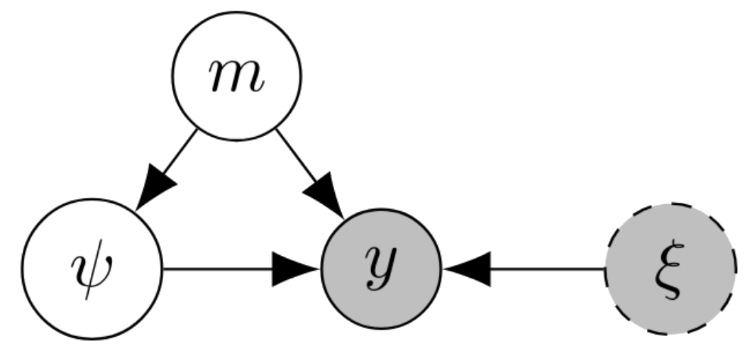
One important feature of the model selection problem is that we do not have a likelihood that directly relates the design \(\xi\), observation \(y\) and the latent variable of interest \(m\). Instead, we have to account for the auxiliary latent variable \(\psi\). We actually have \(p(y\mid m,\xi) = \int_\Psi p(y\mid m,\psi,\xi) p(\psi\mid m) d\psi\).
In this post, we focus on experimental design with the expected information gain (EIG) criterion, also called mutual information utility, that aims to reduce Shannon entropy in our beliefs about \(m\). The EIG-optimal design is specifically,
\[\begin{aligned} \xi^* =\text{argmax}_{\xi} \mathbb{E}_{p(m)p(\psi\mid m)p(y\mid m,\psi,\xi)}\left[ \log \frac{p(m\mid y,\xi)}{p(m)} \right]. \end{aligned}\]Finding \(\xi^*\) amounts to estimating the EIG objective function and optimising over the space of possible designs.
If we have already observed some data \(\mathcal{D}=\{(\xi_1,y_1),\dots,(\xi_T,y_T)\}\), then we fit model-specific posteriors for the auxiliary variable \(\psi\) for each model \(p(\psi\mid m,\mathcal{D})\), and we compute the posterior over models \(p(m\mid \mathcal{D}) \propto p(m)p(\mathcal{D}\mid m)\). Thus, we update our priors \(p(m)\) and \(p(\psi\mid m)\) on the basis of past data.
The variational approach
Posterior lower bound
The general strategy in variational EIG estimation is to optimise variational upper or lower bounds on the EIG. The simplest bound is the posterior lower bound (also called the Barber–Agakov bound after this paper). With the variables we have in this model, the bound would be expressed as
\[\begin{aligned} \mathbb{E}_{p(m)p(\psi\mid m)p(y\mid m,\psi,\xi)}\left[ \log \frac{p(m\mid y,\xi)}{p(m)} \right] \ge \mathbb{E}_{p(m)p(\psi\mid m)p(y\mid m,\psi,\xi)}\left[ \log \frac{q_\phi(m\mid y)}{p(m)} \right]. \end{aligned}\]The new term \(q_\phi(m\mid y,\xi)\) is the amortised approximate posterior with variational parameters \(\phi\). It is an approximate posterior distribution on the latent variable \(m\) of interest. The amortisation here refers to the fact that we learn a function from \(y\) to a distribution over \(m\) (for different \(\xi\), we would train separate functions). For the model selection approach, then, \(q_\phi\) is a function from \(y\) to a distribution over the discrete model indicator \(m\). First, since \(m\) is discrete, the choice of variational family is moot, because every distribution over \(m\) can be finitely represented. Second, \(q_\phi\) has a very simple interpretation. It is a classifier that attempts to predict, on the basis of input \(y\), which model out of \(m_1,\dots,m_k\) generated that data, specifically trying to estimate the posterior probability \(p(m\mid y,\xi)\) over the \(k\) different possibilities for \(m\). Importantly though, rather than just attempting to predict the correct model that was responsible for generating the data \(y\), it is essential that we have probabilistic classifier that assigns probabilities to each possible model. For this probabilistic classifier, the issue of calibration becomes central, as we hope that our classifier probabilities will approach \(p(m\mid y,\xi)\) during training.
We have established that \(q_\phi\) is simply a probabilistic classifier for the model selection case. How should this classifier be trained? In general, our original paper, we proposed training \(q_\phi\) by gradient descent to maximise the lower bound with respect to \(\phi\)
\[\begin{aligned} \phi^* = \text{argmax}_\phi \mathbb{E}_{p(m)p(\psi\mid m)p(y\mid m,\psi,\xi)}\left[ \log \frac{q_\phi(m\mid y)}{p(m)} \right] \end{aligned}\]In model selection, training \(\phi\) simply means training the parameters of the classifier. Maximising the posterior lower bound is equivalent to simply maximising the expected log likelihood under \(q\), i.e.
\[\begin{aligned} \phi^* = \argmax_\phi \mathbb{E}_{p(m)p(\psi\mid m)p(y\mid m,\psi,\xi)}\left[ \log q_\phi(m\mid y) \right]. \end{aligned}\]This is true because \(p(m)\) has no dependence on \(\phi\). So, we see that training \(q_\phi\) to maximise the variational posterior lower bound amounts to maximum likelihood training of a neural classifier when we are in the setting of model selection. (Care may be needed to ensure the classifier produces good probabilistic uncertainty, as well as getting good predictions, as these probabilities are central to our method.)
In fact, we have an enhanced setting in which we can draw an infinite amount of training data by simulating from \(p(m)p(\psi\mid m)p(y\mid m,\psi,\xi)\). To do this, we sample a random model \(m\) from its prior, then a random set of parameters \(\psi \sim p(\psi\mid m)\) for the chosen model, and then simulate an experimental outcome under design \(\xi\). Importantly, we do not need to draw a fixed training or test set, and we never need to show the classifier the same examples twice, we instead draw new batches on the fly. One particularly important consequence of this is that the spectre of over-fitting is much reduced in our case, as there is no fixed training set to overfit to.
We now see another important point—the negative log-likelihood loss of the classifier is essentially an estimate of the EIG, up to a constant. Suppose we have completed training and reached parameters \(\hat{\phi}\). Then the EIG estimate is
\[\begin{aligned} \text{EIG}(\xi) \approx \mathbb{E}_{p(m)p(\psi\mid m)p(y\mid m,\psi,\xi)}\left[ \log \frac{q_{\hat{\phi}}(m\mid y)}{p(m)} \right] = \mathbb{E}_{p(m)p(\psi\mid m)p(y\mid m,\psi,\xi)}\left[ \log q_{\hat{\phi}}(m\mid y) \right] + H[p(m)] \end{aligned}\]and we can estimate the expectation with new, independent batches simulated from the model.
In summary, the posterior lower bound method for model selection amounts to training a classifier on (infinite) simulated data to predict \(m\) from \(y\). The optimal design \(\xi^*\) will be approximated by the classifier which has the best (lowest) validation loss, which is a good approximation of having the highest EIG.
Marginal + likelihood estimator
The posterior lower bound is not the only way to estimate the EIG. Both the marginal and the VNMC methods require an explicit likelihood, so they are not suitable for the model selection scenario. The marginal + likelihood estimator is
\[\begin{aligned} \text{EIG}(\xi) \approx \mathbb{E}_{p(m)p(\psi\mid m)p(y\mid m,\psi,\xi)}\left[ \log \frac{q_\ell(y\mid m,\xi)}{q_p(y\mid \xi)} \right]. \end{aligned}\]This estimator translates, with some simplification, into the model selection setting. The ‘approximate likelihood’ \(q_\ell(y\mid m,\xi)\) in the model selection setting is an approximation of the model evidence \(q_\ell(y\mid m,\xi) \approx p(y\mid m,\xi)\). For model selection when \(m\) is discrete, we do not need to separately estimate \(q_p\) and \(q_\ell\), we can instead sum over \(m\) to obtain
\[\begin{aligned} q_p(y\mid \xi) = \sum_m p(m) q_\ell(y\mid m,\xi). \end{aligned}\]As shown in Appendix A.4 of the VBOED paper, the estimator actually becomes a lower bound
\[\begin{aligned} \text{EIG}(\xi) \ge \mathbb{E}_{p(m)p(\psi\mid m)p(y\mid m,\psi,\xi)}\left[ \log \frac{q_\ell(y\mid m,\xi)}{\sum_{m'} p(m') q_\ell(y\mid m' ,\xi)} \right] \end{aligned}\]on the EIG in this case, which is not generally the case for the marginal + likelihood method. (In fact, this lower bound is itself a special case of the likelihood-free ACE lower bound. If we take the prior as the variational posterior and let \(L\to\infty\) in the LF-ACE bound, we recover this lower bound.)
This lower bound also has a nice interpretation in the model selection scenario. The best design will be the one where the lower bound is largest, which happens, loosely speaking, when \(q_\ell(y\mid m,\xi)\) is much larger than \(\sum_m p(m) q_\ell(y\mid m,\xi)\). That means the approximate model evidence for the observation \(y\) under the correct model \(m\) is much larger than its evidence under other models. Thus, using the experiment with design \(\xi\) and observing \(y\) will allow us to easily discriminate between models.
To explicitly use this method, we need to choose trainable density estimators for \(q_\ell(y\mid m,\xi; \phi)\) with parameters \(\phi\). The simplest method would be to have a distinct set of variational parameters for each value of \(m\) and \(\xi\). Whilst it is possible to use a Gaussian density model, we could use more sophisticated methods such as normalising flows. The training approach is similar to that for the posterior method. We use infinite simulated data, and maximise the variational lower bound using stochastic gradient optimisers.
The last two sections highlight a general feature of variational methods—we can either make variational approximations to densities over \(m\) or over \(y\). Both lead to valid bounds.
Stochastic gradient optimisation of the design
So far, we have focused on variational estimation of the EIG. It is only a short jump from variational estimation of the EIG to stochastic gradient optimisation of the design using a variational lower bound on EIG. The benefit of doing this is that we do not have conduct a grid search, co-ordinate exchange or similar algorithm over the design space. What we require instead is a continuous design space and the ability to differentiate observations with respect to designs.
In our paper on gradient-based experimental design, we introduced several EIG lower bounds which can be used for simultaneous optimisation of the design and variational parameter. Of these, both the posterior (Barber–Agakov) lower bound and the LF-ACE bound are applicable to the model selection setting. There is just one thing to check, which is that we can compute a derivative \(\partial y/\partial \xi\). This is usually fine. For example, if \(p(y\mid m,\psi,\xi)\) takes the form \(y = g(m,\psi,\xi,\epsilon)\) for a differentiable \(g\) and an independent noise random variable \(\epsilon\).
Assuming this is the case, we can train \(\xi\) by stochastic gradient using either the posterior bound or the simplified marginal + likelihood bound. We focus on the posterior lower bound for simplicity. Recall that, for the posterior bound, we are training a classifier to predict \(m\) from \(y\). We have
\[\begin{aligned} \text{EIG}(\xi) \ge \mathbb{E}_{p(m)p(\psi\mid m)p(y\mid m,\psi,\xi)}\left[ \log q_\phi(m\mid y) \right] + H[p(m)] \end{aligned}\]where \(q_\phi\) is the classifier. One thing that we skimmed over slightly in the previous section was that \(\phi\) implicitly depends on \(\xi\) via the training data, and different \(\xi\) will have different classifiers with different optimal values of the classifier parameters \(\phi\).
Rather than training separate classifiers with different designs \(\xi\), the stochastic gradient BOED method updates \(\xi\) and \(\phi\) togther in one stochastic gradient optimisation over the combined set of variables \((\xi,\phi)\). To explicitly write down the \(\xi\) gradient here, let’s assume that we do have \(y = g(m,\psi,\xi,\epsilon)\), so we can write
\[\begin{aligned} \mathcal{L}(\xi,\phi) = \mathbb{E}_{p(m)p(\psi\mid m)p(\epsilon)}\left[ \log q_\phi(m\mid g(m,\psi,\xi,\epsilon)) \right] + H[p(m)]. \end{aligned}\]In this form, the \(\xi\) gradient can be simply calculated as
\[\begin{aligned} \frac{\partial \mathcal{L}}{\partial \xi} = \mathbb{E}_{p(m)p(\psi\mid m)p(\epsilon)}\left[ \left.\frac{\partial \log q_\phi}{\partial y}\right\vert_{m,g(m,\psi,\xi,\epsilon)}\left.\frac{\partial g}{\partial \xi}\right\vert_{m,\psi,\xi,\epsilon} \right]. \end{aligned}\]The beauty of modern auto-diff frameworks, of course, means that we do not even need to calculate this explicitly ourselves.
For model selection, this gradient has a natural interpretation. We want to increase the lower bound \(\mathcal{L}\) by moving to regions in which the classifier can confidently predict the correct model label \(m\). This corresponds to moving \(y\) into regions in which \(\log q_\phi(m\mid y)\) is larger for the model that actually generated \(y\). In other words, we want the input to the classifier \(y\) to be pushed to regions where the classifier already finds it easy to classify correctly. That is, regions where deciding which model is correct is easier. We then exploit the differentiable relationship between \(\xi\) and \(y\), and use this signal to `improve’ the input to the classifier by adjusting the design \(\xi\) to that such datasets \(y\) are more likely to be synthesised.
At the same time, we are constantly making gradient updates on the classifier parameters \(\phi\). This means that, as the distribution of \((m,y)\) changes, the classifier can adjust accordingly.
If this sounds dubious, it is worth taking a step back. We are quite simply optimising the lower bound \(\mathcal{L}(\xi,\phi)\) jointly with respect to \(\xi\) and \(\phi\), in the hopes that this global maximum may closely correspond to the EIG maximiser \(\xi^*\). We actually have a guarantee that the value of \(\mathcal{L}\) at our final trained variables \(\hat{\xi},\hat{\phi}\) is a lower bound on \(\text{EIG}(\hat{\xi})\), i.e.~the true value of \(\hat{\xi}\) cannot be worse than the value we estimate for it.
Whilst the method is approximate, because we cannot quantify the discrepancy between \(\mathcal{L}\) and the true EIG, it is highly scalable to very large design spaces. We also introduced the evaluation method of establishing lower and upper bounds on chosen designs. This numerically bounds the discrepancy between the training objective \(\mathcal{L}\) and the true EIG objective. Sadly, the upper bounds are only valid for explicit likelihood models; they don’t work in the model selection case.
Finally, all of the above discussion carries over if we were to use the marginal + likelihood loewr bound instead of the posterior bound.
Comparing with other classification approaches
We have established that the variational posterior approach to doing Bayesian experimental design for model selection instructs us to learn a classifier to predict \(m\) from \(y\) and use the log probabilities \(q_\phi(m\mid y)\) to estimate EIG. Other authors have considered supervised classification as a means to perform Bayesian experimental design for model selection.
Here, we focus on Hainy et al. (2018), which is “the first approach using supervised learning methods for optimal Bayesian design.” This method trains a classifier that predicts \(m\) using \(y\), with separate classifiers for different \(\xi\). They focus on training decision trees and random forest classifiers. Since random forests are not generally trained by stochastic gradient methods, this means that they fall back on simulating fixed training and test datasets of samples \((m_j, y_j)_{j=1}^J\) from \(p(m)p(\psi\mid m)p(y\mid m,\psi,\xi)\). The training dataset is used to train the classifier model, whilst the test dataset gives unbiased estimates of the posterior loss. There is a danger that the classifier may overfit to the training set in this case. Compare this with the training of stochastic gradient classifiers in our previous sections—here we can draw fresh training batches on the fly, and avoid overfitting to a training set.
Decision trees and random forests do provide estimates of the class probabilities \(q(m\mid y)\), but they are relatively noisy. For this reason, Hainy et al. (2018) focus on the 0–1 loss to evaluate designs. In the language of classification, therefore, they choose the design which gives the best test accuracy. Again, this is different to the variational approach which fits a neural classifier that automatically provides smooth probability estimates \(q_\phi(m\mid y)\). The latter case was applied to estimate the information gain, which we showed is equivalent to choosing the design which gives the best test loss, assuming a negative log-likelihood loss function.
The trade-offs between these methods are clear when we consider optimising over a large design space. For the variational method, we have to train a number of neural networks to convergence. For the classification approach of Hainy et al. (2018), we train a number of random forest classifiers—this may be significantly more computationally efficient. Hainy et al. (2018) propose embedding their 0–1 loss estimation within a co-ordinate exchange algorithm (Meyer and Nachtsheim, 1995) to optimise over designs. The variational method, on the other hand, can naturally be embedded in a unified stochastic gradient optimisation to find the optimal design through stochastic gradient optimisation. The former may be more effective when the design space is not continuous, the latter can work well in a high-dimensional design space that is difficult to search using discrete methods.
Citation
This post is an edited version of Section 7.1 from my thesis. If you’d like to cite it, you can use
@phdthesis{foster2022thesis,
  Author = {Foster, Adam},
  Title = {Variational, Monte Carlo and Policy-Based Approaches to Bayesian Experimental Design},
  school = {University of Oxford},
  year={2022}
}
References
Markus Hainy, David J Price, Olivier Restif, and Christopher Drovandi. Optimal bayesian design for model discrimination via classification. arXiv preprint arXiv:1809.05301, 2018.
Adam Foster, Martin Jankowiak, Elias Bingham, Paul Horsfall, Yee Whye Teh, Thomas Rainforth, and Noah Goodman. Variational Bayesian Optimal Experimental Design. In Advances in Neural Information Processing Systems 32, pages 14036–14047. Curran Associates, Inc., 2019.
Adam Foster, Martin Jankowiak, Matthew O’Meara, Yee Whye Teh, and Tom Rainforth. A unified stochastic gradient approach to designing bayesian-optimal experiments. In International Conference on Artificial Intelligence and Statistics, pages 2959–2969. PMLR, 2020.
David Barber and Felix Agakov. The IM algorithm: a variational approach to information maximization. Advances in Neural Information Processing Systems, 16:201–208, 2003.
Ruth K Meyer and Christopher J Nachtsheim. The coordinate-exchange algorithm for constructing exact optimal experimental designs. Technometrics, 37(1):60–69, 1995.